Tractor Insurance Policy Using GLM
Developmet and evaluation of an insurance policy for tractors using a generalized linear model
The insurance for tractors in Europe is heavily dominated by a few large companies. The goal with this project is goal to create an insurance policy which would profit and perform well on the market. A Generalized Linear Model (GLM) was used to achieve this goal together with a dataset contining historic information about tractors and the insurance claims related to the tractors.
Analyses and model development
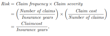
We will use linear regression to develop our insurance policy where we can calculate the risk of our customers, so that we know what each customer should pay. The risk can be calculated accordingly to the formula in figure 1. The risk that we calculate is strictly a positive value, since we cannot give people money for signing up for an insurance with us. The outputs of our model is therefore assumed to be Poisson distributed. The Poisson distribution is part of the exponential family which is convenient to model with Generalized Linear Models. The Log link function is used since it has been shown to work with Poisson distributions and is often the default link function for such distributions. We furthermore know, as seen in figure 1, that the risk can be decomposed into two models, where one is used for calculating the claim frequency and the other one is used for calculating the claim severity.
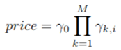
Another convenience with the log link function is that the price can be calculated as a product of factors, as seen in figure 2 where the factors \(\gamma_{k,i}\) are fixed values for the features that are included in our model, such as geographic location etc., and \(\gamma_0\) is a base level that the product of factors should be multiplied with to get the correct price. This makes it easier for both customers and employees to calculate how the price changes depending on the features of the tractor. Since the model factors for each model are multiplied together, we use the same regressors for both of the models.
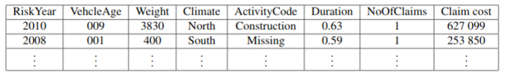
In order to build a GML, we need data. If P&C insurance has provided a data set of tractor insurance customers which consist of collected data between year 2006-2016. The data set includes information such as the vehicle age, weight, location, use case, how long the insurance lasted, number of claims and claim costs. An example of a database record can be found in figure 3. As we can see, some of the values are continuous, and since we build a GLM with categorical data, we have to group our continuous data. We therefore create groupings of the data which are risk homogeneous and have enough data. We then fit the General Linear Model according to the different groupings.
Grouping of data
Weight: When creating groups for the weight class we had the assumption that the use case for the tractor has a connection to the weight of the tractor, and that tractors with the same use case should have similar risk. Initial research was done on what kind of tractors exist in the market right now. We found a tractor manufacturer called John Deere. John Deere product catalog is divided depending on the size of the tractors, and therefore the weight for every size-group of the tractors was collected. With the collected information, weight intervals for the different groups were created as a start.
In addition to this, the raw data in the data set was investigated manually. We discovered that there existed some invalid values and therefore a group for invalid values was added.
After creating the initial groupings, the distributions of the data given the grouping was investigated. It was shown that the group for the lightest tractor had approximately double the size compared to the other groups. Therefore, it was investigated if it was plausible to further divide that group. The data in the lightest group was ordered and plotted and we discovered that there existed tractors that were significantly lighter than expected, which we assumed are either invalid values or that there existed an even lighter group of tractors than we anticipated. After research it was found it does indeed exist a group of even lighter tractors, therefore the groupings were changed. The intervals were finally manually tuned, while keeping an eye on the AIC score. This was an iterative process and we settled on the final intervals for the weights: (-Inf,199), (200, 499), (500, 1249), (1250, 2999), (3000, 5999), (6000 ,9999), (10000, Inf).
Age: When creating the grouping of the age group we used the intuition that in the beginning of the tractors life, the risk of breaking down is higher, and the older the tractor becomes the lower risk becomes. Eventually the risk should plateau. The intuition is inspired by natural selection, that is tractors that have good quality reach older ages. There was also a group added for values that seems to be invalid. The distribution of data in the groups was investigated and it was found sufficient. The final intervals for the age classes are (-Inf, 2), (3, 7), (8, 14), (15, 44), (45, Inf).
Measure goodness of fit
Now that we have our data in classes, we can use them to fit our Generalized Linear Models. Our final model is a product of two separate models which predicts the frequency of claims and the severity of the claims. A likelihoodratio test is done on both of the models where each model (Full models (FM)) is compared to the reduced models (RM) were each of reduced model has one of the explaining variable removed.
| Removed variable | P-value |
|---|---|
| Age | 0.04239808 |
| ActivityCode | 6.794081e-05 |
| Climate | 6.553373e-05 |
| Weight | 1.546386e-29 |
| Removed variable | P-value |
|---|---|
| Age | 4.807923e-19 |
| ActivityCode | 7.918679e-09 |
| Climate | 0.5293175 |
| Weight | 7.659316e-33 |
The results of the likelihood ratio tests can be seen in table 1 and table 2. We can see that the p-value is under 0.05 for all the different tests except the one were the reduced frequency model didn't have the climate variable, which could be a sign that the climate variable should be removed from the final model. However if we look at the p-value for the same test but for the severity model we can see that the p-value is very low and due to the constraint that both models should have the same explaining variables we decided to not remove any variables from the final model.
Calculating the base level
Now that we have our risk factors \(\gamma_{k,i}\) from the equation in figure 2, we have to determine the base level \(\gamma_{0}\) using only data from the insurances that are active today. The purpose of this is to set our base level so that the price for the insurance each year covers the predicted claim cost.
The goal is to estimate the damage cost for 2017, one way to do this is to assume that it is exactly the same as 2016. The damage cost for 2016 need to be calculated as if all insurance policies were valid all year, so we divide this cost with total duration for 2016. The cost needs to be adjusted to take into account a margin which is needed to cover our cost and make a profit. With a premium of 90% (which we used), the estimated claim cost for 2017 needs to be divided by 0.9.
Now the relative risk for each insurance needs to be calculated. This is done by multiplying the risk factors that are relevant for the tractor of each data point from 2016, this is called the total relative risk. The total relative risk is then summarized for the entire portfolio. The sum received will differ from the total premium by a certain factor, this is the base level.
Results
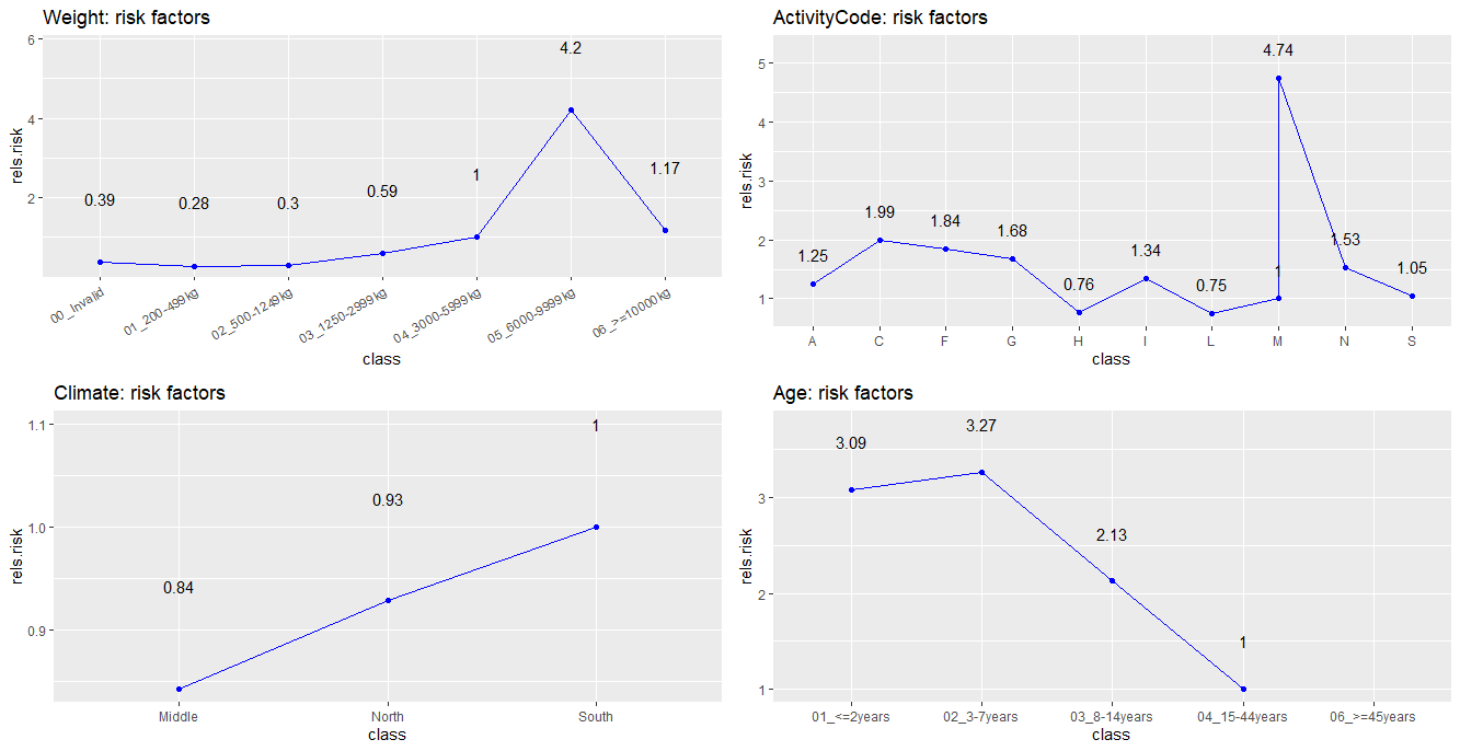
For our final model, we got the the final risk factors in figure 4. We can see that some factors are very large in relation to the others, and our theory for this is that these factors is the effect of extreme data values. We decided to not remove any data since they are still part of the expected cost. Removing them means that we are ignoring some costs that affects the resulting insurance policy, which can cause us to lose money each year. Otherwise, they seem reasonable. One could for example expect the risk to increase with increasing weight. The base level \(\gamma_{0}\) for our insurance policy had the final value of 205. This value and the corresponding risk factors for our tractors are inserted into the equation in figure 2 to calculate the price. This is our final insurance policy that we deliver to the investor.
Conclusion
We built a GLM model to produce our insurance policy using data from If P&C insurance. The risk was decomposed into claim frequency and claim severity which were assumed to be Poisson distributed. We could therefore model the insurance policy as products of risk factors. In the end we could conclude that the values of the risk factors for our final models captures some of the intuitions that exists when thinking about how the risk should reflect the given tractor. A risk base level was calculated to ensure some profit each year, with a premium of 90%. Hopefully this insurance policy will lead to a profitable business in the European market.